EL LEGADO DE ALAN TURING / THE LEGACY OF ALAN TURING
ALAN TURING AND THE ORIGINS OF COMPLEXITY
Miguel-Angel Martin-Delgado
Departamento de Física Teórica I, Universidad Complutense
mardel@miranda.fis.ucm.es
ABSTRACT
The 75th anniversary of Turing’s seminal paper and his centennial anniversary occur in 2011 and 2012, respectively. It is natural to review and assess Turing’s contributions in diverse fields in the light of new developments that his thought has triggered in many scientific communities. Here, the main idea is to discuss how the work of Turing allows us to change our views on the foundations of Mathematics, much as quantum mechanics changed our conception of the world of Physics. Basic notions like computability and universality are discussed in a broad context, placing special emphasis on how the notion of complexity can be given a precise meaning after Turing, i.e., not just qualitatively but also quantitatively Turing’s work is given some historical perspective with respect to some of his precursors, contemporaries and mathematicians who took his ideas further.
ALAN TURING Y LOS ORÍGENES DE LA COMPLEJIDAD
RESUMEN
El 75 aniversario del artículo seminal de Turing y el centenario de su nacimiento ocurren en 2011 y 2012, respectivamente. Es natural revisar y valorar las contribuciones que hizo Turing en campos muy diversos a la luz de los desarrollos que sus pensamientos han producido en muchas comunidades científicas. Aquí, la idea principal es discutir como el trabajo de Turing nos permite cambiar nuestra visión sobre los fundamentos de las Matemáticas, de forma similar a como la mecánica cuántica cambió nuestra concepción de la Física. Nociones básicas como compatibilidad y universalidad se discuten en un contexto amplio, haciendo énfasis especial en como a la noción de complejidad se le puede dar un significado preciso después de Turing, es decir, no solo cualitativo sino cuantitativo. Al trabajo de Turing se le da una perspectiva histórica en relación a algunos de sus precursores, contemporáneos y matemáticos que tomaron y llevaron sus ideas aún más allá.
Recibido: 10-07-20132; Aceptado: 15-09-2013.
Citation/Cómo citar este artículo: Martin-Delgado, M. A. (2013). "Alan Turing and the Origins of Complexity". Arbor, 189 (764): a083. doi: http://dx.doi.org/10.3989/arbor.2013.764n6006.
PALABRAS CLAVE: Máquina de Turing; Computabilidad; Complejidad Algorítmica; Complejidad Computacional; Clases de Complejidad; Omega de Chaitin; Entropía Algorítmica; Barrera de Turing.
KEYWORDS: Turing Machine; Computability; Algorithmic Complexity; Computational Complexity; Complexity Classes; Chaitin Omega; Algorithmic Entropy; Turing Barrier.
Copyright: © 2013 CSIC. This is an open-access article distributed under the terms of the Creative Commons Attribution-Non Commercial (by-nc) Spain 3.0 License.
CONTENTS
I. INTRODUCTION Top
At the year of this writing, 2011, it is 75 years since the seminal paper by Alan Mathison Turing (Turing, 1936Turing, A. M. (1936). "On computable numbers, with an application to the Entscheidungsproblem". Proc. London Math. Soc., {[2]} 42 (1936-37), 230-265; Correction, ibid., 43 (1937), 544-546. Online open access http://www.abelard.org/turpap2/tp2-ie.asp.) was published. And 2012 will mark the centenary of his birth. This looks like a good occasion to review and assess his work and impact and to See how useful and vital it has become in so many aspects and disciplines. As time goes by, the importance and relevance of Turing’s seminal paper rises. Turing transcends Mathematics and goes into other disciplines like Physics, Engineering, etc. His work started as an in-depth study of the very notion of what an algorithm is, discarding what was irrelevant and targeting the essence of a mechanical procedure with a new notion of a theoretical machine. This very simple machine, the Turing machine, however turns out to be extremely powerful and even universal. In this regard, Turing’s work parallels Einstein’s on special relativity, when Einstein went to make precise and explicit definitions of elementary concepts like distances, time intervals, clock synchronization and the definition of an inertial frame. Despite their simplicity, however the consequences of Einstein’s principles revolutionized the whole of Physics. Turing’s work is of a similar kind.
Turing made a gigantic effort to understand how the human mind works at the level of finding mechanical procedures to compute things and devise appropriate definitions of what algorithms are (Turing, 1936Turing, A. M. (1936). "On computable numbers, with an application to the Entscheidungsproblem". Proc. London Math. Soc., {[2]} 42 (1936-37), 230-265; Correction, ibid., 43 (1937), 544-546. Online open access http://www.abelard.org/turpap2/tp2-ie.asp.). His work represents a great deal of imagination and creativity, which in turn has changed the notion of creativity ever since, for creativity now can be made quantitative using Turing’s work.
He invented the theory of computability. What is more important, this affects the way Mathematics must be understood at a fundamental level, the calculus. And he did more. His results have revolutionized the way we address axioms, i.e., the very fundamentals of Mathematical disciplines. He addressed questions such as when a set of axioms is complete, what to do when it is not. Ultimately, this leads to the very notion of mathematical creativity.
Turing has achieved considerable recognition in Engineering Schools, such as Computer Science and many others. However, it is rather disappointing to see that the figure of Turing and his work still does not have a central, pivotal role in the curricula of university mathematics departments, a fact which merits a word or two. Firstly, Turing’s theory can be regarded as the fundamental to what a calculation should be in Mathematics. It underlines all previous knowledge on calculus and analysis in Mathematics in a way that was implicit before Turing. After Turing, it is systematized in a way that it becomes mechanical and algorithmic: the holy grail of any theory. Secondly, it affects the way axioms have to be considered in Mathematics. The big surprise is that Mathematics is not closed in the sense predicted by David Hilbert, but it is an open system capable of increasing its amount of knowledge by adding new axioms to a discipline.
And the same goes for university physics departments, where the computer science part of in the curricula is mostly reduced to learning manuals of software instead of the fundamentals of computation. Manuals are changeable, version after version, but Turing’s foundations on computability theory remain.
Turing’s work has led to the development of 3 major disciplines:
Computability: it studies which problems can be computed and which cannot be computed. This goes to the very limits of what is knowable.
Complexity: once a problem is computable or solvable, then we need to know how difficult is to compute it. This can be quantified in various ways giving rise to different notions of complexity: algorithmic complexity, computational complexity and others that will be considered in Sect. III, VI.
Universality: the new paradigm is to use a TM, the basis of a real computer, in order to solve problems. Then, we need to know how general these machines, Turing machines, can be. Does every problem or reduced set of them require a particular TM? This is another fundamental discovery, the notion of a Universal Turing Machine (UTM): a machine that can simulate the functioning of any other TM. Here it is important to study how many resources we need to create such a UTM.
These disciplines are part of computer science as envisaged by Turing and extend to many branches of science like Physics, Mathematics, Engineering, etc. This extension will increase with our better understanding of Nature and will apply to more descriptive sciences like Biology.
From Turing’s work it is apparent that with a finite set of axioms it is not possible to cover Mathematics as a whole. There are irreducible truths, axioms that are not self-evident in the sense of Euclid or Hilbert, and must be added to as independent axioms. This makes a TOE (Theory of Everything) of Mathematics impossible.
II. WHAT YOU CAN COMPUTE... Top
Turing was the first to separate software from hardware in a very concrete way. He did that by first focusing on the theoretical problem of having a well-defined notion of a computing machine. In his later years, he also got involved in constructing computing machine in practice (Turing, 1946Turing, A. M. (1946). "Proposed Electronic Calculator" (ACE), National Physical Laboratory internal document (1946). The original copy is in the (British) National Archives, in the file DSIR 10/385. first published as the NPL report, Com. Sci. 57 (1972), with a foreword by Donald W. Davies.).
Turing first goal was to scrutinize all steps that a person realizes during a calculation, like arithmetic, and separate irrelevant aspects from the relevant properties necessary to carry out the calculation. In doing so, he realized that there were two main ingredients: ‘local information’ and ‘state of mind’. Local information means that at each calculation step, only a small part of the whole operation is being performed. State of mind means that the steps after a local calculation is carried out, depend on the rules stored in the person’s mind which defines the calculation itself. Turing realized that it was enough to use a one-dimensional roll of paper or pad to write the intermediate (local) calculations and that the rules of the state of mind could be also stored in a table of operations. After this analysis, Turing came up with an abstract construct of his machine.
Turing Machine: it is a finite-state machine with 3 components: i/ a doubly-infinite one-dimensional tape where symbols from an alphabet were written or read from square cells; ii/ a control unit that stores the set of instructions in a table of specific operations; iii/ a head that scans one cell of the tape at a time and reads or writes alphabet symbols onto the tape depending on the instructions in the control unit. A more formal mathematical definition with the concrete functioning, examples and diagrams can be found in (Galindo, Martin-Delgado, 2002Galindo, A. and Martin-Delgado, M. A. (2002). "Information and Computation: Classical and Quantum Aspects". Rev.Mod.Phys., 74, pp. 347-423.).
He was so convinced that this definition of machine represented the most general possible algorithm for calculus that he formulated the basic principle of computation by means of his construction:
Turing Hypothesis: (also known as the Church-Turing thesis):
“A function is computable, if and only if, it can be computed by a Turing machine.”
Turing named his machine 'a-machine' for automatic machine (Turing, 1936Turing, A. M. (1936). "On computable numbers, with an application to the Entscheidungsproblem". Proc. London Math. Soc., {[2]} 42 (1936-37), 230-265; Correction, ibid., 43 (1937), 544-546. Online open access http://www.abelard.org/turpap2/tp2-ie.asp.). In essence, this statement is more than a mathematical axiom, it is part of Physics as it is a principle that tells us what we can compute in our Universe.
A basic and fundamental result of the notion of a TM is that the set of TMs is countable, infinitely denumerable. It corresponds to bit-strings. Let  := {Λ, 0, 1, 00, 01,10,11, 000, ...} be the set of finite strings of binary bits, with Λ denoting the blank space symbol. The size or number of bits is |x|. The set of infinite bit-strings is denoted as
  . A Turing Machine TM is an application T: x → that takes an input data q ∈ and a program p ∈ that acts on the input to produce an output string T(p, q) = x ∈ which is the result of the computation, assuming it halts. When the input data is empty, we simply write T(p) = x, and when the output is simply stopping the computer with no output, we write T(p) : halts.
However, the notion of a TM is tight to the computation of a given function or problem. Changing the function means changing the TM. Here comes the notion of universality as a property of a special TM that can compute what any other TM can do.
Universal Turing Machine: denoted as UTM, it is a construction based on set of instructions and states in the control unit of a TM such that it can reproduce the functioning of any other TM.
It is very remarkable that the definition of a TM allows for this property of universality. The basic idea behind the UTM is the observation that a TM T can be described by a bit-string itself and supplied to another TM T* along with input data q ∈ . Thus, T* (T, q) will produce the same result as T(q), thereby T* simulating the functioning of any TM
T.
In doing so, Turing was giving birth to programming and compiling. A universal TM is the notion of a general-purpose programmable computer today. After Turing gave the first construction of a UTM (Turing, 1936Turing, A. M. (1936). "On computable numbers, with an application to the Entscheidungsproblem". Proc. London Math. Soc., {[2]} 42 (1936-37), 230-265; Correction, ibid., 43 (1937), 544-546. Online open access http://www.abelard.org/turpap2/tp2-ie.asp.), other constructions have been presented depending on the number of states used by the machine and the number of symbols in the alphabet (Shannon, 1956Shannon, C. E. (1956). "A Universal Turing Machine with Two Internal States". In Automata Studies. Princeton, NJ: Princeton University Press, pp. 157-165.; Minsky, 1962Minsky, M. L. (1962). "Size and Structure of Universal Turing Machines Using Tag Systems". Proc. Sympos. Pure Math., 5, pp. 229-238.), including small ones (Rogozhin, 1996Rogozhin, Y. (1996). "Small Universal Turing Machines". Theoret. Comput. Sci., 168, pp. 215-240.).
Von Neumann realized that Turing had achieved the goal of defining the notion of universal computing machine, and went on to think about practical implementations of this theoretical computer. It was clear that this was the crucial notion of a flexible computer that was needed and was lacking thus far. Therefore, the distinction between software and hardware is clear in Turing’s work and it is a consequence of it. Turing did not care about practical implementations at his time because he wanted to isolate, to single out the very notion of what a computer is, in theory. In doing so, he was inspired by D. Hilbert and his ideas about a formal set of axioms from which theorems would be provable by means of a mechanical procedure. This led to the notion of TM and the solution of Hilbert’s tenth problem.
As the title of his 1936Turing, A. M. (1936). "On computable numbers, with an application to the Entscheidungsproblem". Proc. London Math. Soc., {[2]} 42 (1936-37), 230-265; Correction, ibid., 43 (1937), 544-546. Online open access http://www.abelard.org/turpap2/tp2-ie.asp. paper states, Turing wanted to give a concrete definition of what a computable real number is. By introducing the TM, he identified computable numbers with those that a TM can really compute. Thus, a real number is computable when its decimal digits are computable by finite means.
Computable Numbers: a real number x ∈ R is a computable real if there exists a computable function T(k), k ∈ N such that x is bounded by rational numbers:
Fortunately, all algebraic numbers, as well as, π, e, and many other transcendental numbers are computable reals.
In addressing non-computable problems in Sect.III, it is useful to introduce a variant of Turing machine due to Chaitin (Chaitin, 1975Chaitin, G. J. (1975). "A theory of program size formally identical to information theory". J. ACM, 22, pp. 329-340.; Chaitin, 1987Chaitin, G. J. (1987). Algorithmic Information Theory. Cambridge University Press.).
Chaitin Machine: it is a self-delimiting or prefix-free Turing Machine, denoted CM.
This means that the TM knows when to stop by itself, without needing a special mark indicator or blank character. Formally, it is an application C: x → that is a TM acting on programs p ∈ and input data q ∈ , such that both p and q are self-delimiting strings, also called prefix-free. A set of strings  ⊂ is prefix-free if ∀s, s’ ∈ , s is not included as a prefix in s’. For example, the set of all bit strings up to size 2,
  := {0, 1, 01, 10} is not prefix-free for 0 is prefix of 01. However, = {0, 10} is prefix-free.
An explicit construction of a Chaitin machine is as follows. It has three elements: i/ a finite program tape; ii/ a doubly-infinity work tape; iii/ a head with one arrow scanning the program tape and another arrow scanning the work tape. The alphabet is binary 0, 1 and the blank space is not allowed to mark the halting of the machine. The initial state of a CM is the program p ∈ stored in the program tape and with the arrow head scanning the left-most square which is blank. As for the work tape, it is occupied with the input data q ∈ and the arrow head is scanning the left-most bit (initial bit) of q. After the initial state, the CM starts operating like a TM: the arrow head only moves on the program tape to the right, while the arrow head can move left/right on the work tape; the arrow head can read and erase the square of the work tape being scanned. The CM will halt if the arrow head reaches the right-most square of the program tape, giving a certain output result C(p, q) =: x ∈ ; otherwise, C(p, q) is not defined and does not halt. Exactly as with ordinary Turing machines, the CM moves step by step following a previously given finite table that completely determines the computation for the argument (p, q).
Notice that this construction of a TM is self-delimiting since the read arrow head cannot read-off the right-most square of the finite program tape. Also, in an ordinary TM, a program that halts is necessarily prefix-free: it cannot be extended into another program that halts.
Procedures exist to make a given set of bit-strings into a self-delimiting set. For a bit-string x we construct a new bit-string by appending to it a prefix depending on its length |x| =: n as follows:
For instance, from the above we construct  = {010, 011, 00101, 00110} ⊂
  , which is prefix-free. Thus, the length increases only by an additive logarithmic term in the transition from a bit-string to its self-delimiting presentation:
asymptotically. An important property is that universal Chaitin Machines also exist: the universal CM U starts reading a prefix-free program πc that indicates which CM to simulate, followed by the binary program for that machine, U(πcp) = C(p), with p also prefix-free. The whole input program for U can also be made prefix-free.
III. ... AND WHAT YOU CANNOT COMPUTE Top
It is a twist of fate that in the same paper where Turing shows what we can compute in a very precise and universal way ... he also proves that there are things that we cannot compute at all.
Gödel’s theorem on incompleteness (Gödel, 1931Gödel, K. F. (1931). "Fiber formal unentscheidbare Sátze der Principia Mathematica and verwandter Systeme, I". Monatshefte für Mathematik and Physik, 38, pp. 173-98.) was a first shock for the foundations of Mathematics as a complete formal logical system. The latter was the attitude predominant before and well represented by David Hilbert. Yet, the real impact of Gödel’s was still under debate in the Mathematics community and there was the impression that they were a kind of minor anomaly that would not affect the whole building of the theory. Turing’s non-computability results were even more demolishing for the fundamentals of Mathematics since he showed that a very important example of Gödel’s results was also at the heart of computation, algorithmic, something very practical and with a lot of impact in the future.
It is easy to write programs, in pseudocode, that will never halt:
will loop forever. Another less evident example of looping program is:
It produces the cycle 1, 4, 2, 1 forever.
Thus, a skilled debugger may envisage the task of finding all possible loops in programs and with a look-up table, get rid of them. Or maybe, one has to study more and it is necessary to classify families of loops etc. Turing’s proof shows that this dream is impossible and does not depend on how smart the debugger is. It is at the roots of computational theory. In fact, we can guess that the purposed debugger may easily run into unknown territory. For instance, we can use the Collatz conjecture (Collatz, 1937Collatz, L. (1937). Unpublished.) to write the following simple program:
It has been confirmed that this program stops for very large values, n ≤ 20 x 258 (Oliveira e Silva, 2012Oliveira e Silva, T. (2012). Retrieved from http://www.ieeta.pt/ tos/3x+1.html.), but it is unknown whether it halts ∀n ∈ N. The conjecture remains unproven. A modification of it can has been proved to be undecidable (Kurtz, Simon, 2007Kurtz, S. A. and Simon, J. (2007). "The Undecidability of the Generalized Collatz Problem". In Cai, J.-Y.; Cooper, S.B. and Zhu, H. (eds.), Proceedings of the 4th International Conference on Theory and Applications of Models of Computation, TAMC 2007 held in Shanghai, China in May 2007, pp. 542-553.), but the modification does not apply to the original conjecture.
A basic and fundamental result of the notion of a TM is that the set of TMs is countable, infinitely denumerable. It corresponds to bit-strings . This is the power of TMs ... and also its weakness. Although we know that its cardinality is infinity, after Cantor we know that not all infinities are alike. In particular, || is an infinity equal to the infinity of the real numbers N. This is easily obtained by seeing a bit-string as the binary representation of an integer number in base 2:  .
.
Cantor’s diagonal method provides a clever way to see that there are more real numbers R than natural numbers N (Cantor, 1891Cantor, G. (1891). See (Suppes, 1960).; Suppes, 1960Suppes, P. (1972, 1960). Axiomatic Set Theory. New York: Dover.; Dauben, 1979Dauben, J. W. (1979). Georg Cantor: his mathematics and philosophy of the infinite. Boston: Harvard University Press.).
Cantor’s Diagonal Method: it is a technique in set theory to create a new element which is not an element of a previously given set of elements.
As an illustration, consider the following table where we place eight bit-strings := {x1, x2, ... , x8} ⊂ . From this, we can construct another element x9 ∉ G: select the diagonal of the table and negate each of its bits. Then, we get x9 := 00000000 which is new.
The diagonal method is very general. It applies both to finite sets like , or infinite sets like : the set of infinite binary strings. A consequence of this is that has infinite cardinality but it is uncountable. To show this, we proof it by reductio ad absurdum. Assume that is countable so that we make a table like (7) with infinite elements ordered by the integers N. All elements are thus listed, but with the diagonal we can create another bit-string xd:
where xi,i is the ith bit of the ith listed element of . But then, xd ∉ , which is a contradiction. The assumption that was a countable set is not true.
In fact, we can go on and prove that the set of real numbers R is uncountable by establishing a bijection between and R. Both N and R are infinite sets, but of a different quality. The cardinality of N is denoted by ℵ0. R has the cardinality of the continuum.
Continuum Hypothesis (CH): it states that the cardinality of R is ℵ1, the second transfinite cardinal introduced by Cantor, or equivalently, that every infinite subset of R must apply bijectively on either N or on R itself: 2ℵ0 = ℵ1
In other words, there is no set with an intermediate cardinality between N and R, there is a gap. CH was introduced by Cantor but was unable to prove it (Dauben, 1979Dauben, J. W. (1979). Georg Cantor: his mathematics and philosophy of the infinite. Boston: Harvard University Press.). It is the first of Hilbert’s twenty-three problems proposed in 1900. Gödel proved that CH is consistent with axiomatic set theory (Gödel, 1940Gödel, K. F. (1940). The Consistency of the Axiom of Choice and of the Generalized Continuum Hypothesis with the Axioms of Set Theory. Princeton University Press.), but Paul J. Cohen also proved that the negation of CH is also consistent with the axioms of set theory (Cohen, 1963Cohen, P. J. (1963). "The Independence of the Continuum Hypothesis". Proceedings of the National Academy of Sciences of the United States of America, 50 (6), pp. 1143-1148.). Thus, CH is undecidable or non-computable. It is independent of standard axiomatic set theory (Zermelo—Fraenkel set theory).
Non-Computable Numbers: a real number non-computable by a TM.
The set of computable reals with a TM is quite small. Given a TM with |S| internal states, it can compute about (4|S| + 4)2|S| different numbers. Using Cantor’s diagonal method, Turing was able to prove that there are uncountably many noncomputable numbers. Most of the real numbers, the continuum, is inaccessible to a TM.
The diagonal method has proved extremely useful in fundamental problems of Mathematics. Some instances are Russell’s paradox in set theory, Gödel’s first theorem of incompleteness and Turing’s solution to the 10th Hilbert’s problem.
Halting Problem: There is no way to find whether a computer will eventually halt.
A crucial assumption in Turing’s formulation of this problem is that there is no limit for the running time of the computer. By computer is meant a TM. Under these circumstances, there is no mechanical procedure that can decide in advance whether a computer will ever halt. A more formal statement is the following:
Let H be the set of subsets, such that each subset corresponds to a Turing Machines Tn , n ∈ N and all its programs that halt when input on Tn. Each program can also be labelled with an integer m ∈ N. Thus, the allegedly total halting set is
In bit-string notation Tn(m) := Trn (pm, 0), i.e., input data q = 0, the program pm ∈ is the bit-string of the natural number m and similarly for the bit-string xr labelling TMs. Each subset of H is the halting set of a TM Hn:
Now, we are in the situation of applying Cantor’s diagonal method. The set H can be arranged as a table (7), with Hn being the rows. Let us define a ‘diagonal’ set D as follows:
By construction, D is a set of natural numbers that is different from any halting set Hn of any TM. Therefore, the original goal of determining the set H of all halting machines cannot be accomplished and thus, we can never know in general when a TM will ever halt.
Turing did not use the terminology of `halting problem’ in his 1936 paper (Turing, 1936Turing, A. M. (1936). "On computable numbers, with an application to the Entscheidungsproblem". Proc. London Math. Soc., {[2]} 42 (1936-37), 230-265; Correction, ibid., 43 (1937), 544-546. Online open access http://www.abelard.org/turpap2/tp2-ie.asp.). It seems that the first time this was used was by Martin Davis (Davis, 1965; Copeland, 2004Copeland, J. (ed.) (2004). The Essential Turing: Seminal Writings in Computing, Logic, Philosophy, Artificial Intelligence, and Artificial Life plus The Secrets of Enigma. Oxford, UK: Clarendon Press (Oxford University Press).).
After Turing found an explicit and crucial example of a non-computable problem, it was natural to ask whether more examples of this kind could be found. In 1962, T. Radó (Radó, 1962Radó, T. (1962). "On non-computable functions". Bell System Technical Journal, 41 (3), pp. 877-884.) proposed another interesting non-computable function (Galindo, Martin-Delgado, 2002Galindo, A. and Martin-Delgado, M. A. (2002). "Information and Computation: Classical and Quantum Aspects". Rev.Mod.Phys., 74, pp. 347-423.).
Busy Beaver Function: it is the maximum number of digits 1s that appear as output x in a TM T that runs over all programs p that halt on no input q = Λ:
where |x(1)| is the number of 1s in x ∈ . There are several variants of Busy Beaver functions that have the same property of being non-computable and are more manageable definitions. For instance, as the maximum integer number that can be named with a universal TM U with programs of a given size |p| =: N. Thus, a N-th Busy Beaver function is denoted ∑N and defined
This is a well-defined function ∑N : N → N , but it is noncomputable: it grows faster than any computable function ƒ(N), ∑N > ƒ(N) for sufficiently large N. Therefore, ∑N cannot be bounded in the form of ∑N = O(ƒ(N)). The proof goes by reductio ad adsurdum: if it could be bounded, then the halting problem would be computable. More examples of non-computable functions can be obtained systematically by means of the Algorithmic Information Theory (AIT) (Solomonoff, 1964Solomonoff, R. (1964). "A Formal Theory of Inductive In¬ference Part I". Information and Control, 7 (1), pp. 1-22.; Kolmogorov ,1965Kolmogorov, A. N. (1965). "Three Approaches to the Quantitative Definition of Information". Problems Inform. Transmission, 1 (1), pp. 1-7.; Chaitin, 1966Chaitin, G. J. (1966). "On the length of programs for computing finite binary sequences". Journal of the ACM, 13, pp. 547-569.).
After Turing’s halting problem, we may ask: can we quantify non-computability on mathematical grounds? G. Chaitin has done a great deal of work (Chaitin, 1975Chaitin, G. J. (1975). "A theory of program size formally identical to information theory". J. ACM, 22, pp. 329-340.; Chaitin, 1987Chaitin, G. J. (1987). Algorithmic Information Theory. Cambridge University Press.; Chaitin, 2001Chaitin, G. J. (2001). Exploring randomness. London: Springer-Verlag.; Chaitin, 2003Chaitin, G. J. (2003). The Limits of Mathematics. London: Springer-Verlag.) by approaching this issue from information-theoretical methods. He has developed the concept of what it known as Chaitin’s Ω number, which allows us to address this fundamental question. Thus, we need to introduce some basic concepts and results from AIT.
Algorithmic Information Theory (AIT): it is a part of Information Theory that deals with the algorithmic complexity of functions and problems. The algorithmic complexity of a program p ∈ refers to its program-size, i.e., bits of information regardless the run-time that a machine like a TM takes to execute it. It is defined as the shortest program that can reproduce a given string x in a universal TM:
A first consequence of this definition is that H(x) is not computable itself, for two reasons: due to the halting problem, we never know when the programs will halt, and because it is a minimization procedure. Moreover, it is not possible to compute lower bounds to H(x). What is possible is to give the upper bounds. These are good enough to gain a great deal of insight into a given problem. For instance, we can give an alternative definition to the Busy Beaver function:
where the algorithmic complexity (14) is defined for programs p that compute k = U(p) without input and halting.
Although non-computable, algorithmic complexity is well-defined and it has very useful properties like subadditivity: the joint complexity is bounded by the sum of the complexities of the individuals:
This allows us to construct big programs out of small ones. Another crucial property follows from a proper definition of relative entropy H(y|x)
Thus, the joint complexity of two bit-strings can be computed knowing the absolute complexity of the first one plus the relative complexity of the second given the first one. The key point for this result to hold true is the definition of relative complexity of y given x, H(y|x*): the size in bits of the smallest self-delimiting program for calculating y if we are given for free, not x directly, but x*, a minimum-size self-delimiting program for x.
A fundamental property of Chaitin machines is that they allow us to define halting probabilities for TMs, or the algorithmic probability of a bit-string, also known as universal probability PU(x) of a given string x ∈ :
which is the probability that a program randomly drawn as a sequence of fair coin flips p = p1p2... will compute the string x. This is well-defined thanks to the prefix-free property of CMs and results from AIT (Chaitin, 1975Chaitin, G. J. (1975). "A theory of program size formally identical to information theory". J. ACM, 22, pp. 329-340.; Chaitin, 1987Chaitin, G. J. (1987). Algorithmic Information Theory. Cambridge University Press.; Chaitin, 2001Chaitin, G. J. (2001). Exploring randomness. London: Springer-Verlag.; Chaitin 2003Chaitin, G. J. (2003). The Limits of Mathematics. London: Springer-Verlag.).
A central theorem relates algorithmic complexities with algorithmic probabilities:
This relation tells us that near-minimum size programs for calculating something, elegant programs, are essentially unique. This is a mathematical formulation of Occam’s Razor. Essentially, this relation tells us that AIT is equivalent to Probability Theory, although this probability has to do with randomness in programs, rather than statistical randomness but we shall get back to this later.
The idea behind structural or logical randomness is lack of structure or pattern in a program or bit-string. Thus, a program or bit-string is random if it has no pattern or inner structure, consequently, it cannot be compressed. The only way to address it is by printing the whole program as it is: there is no theory behind it from which it can be derived. By theory, we mean a simpler procedure to recover the bit-string, i.e. something compressible. Now, we can give a precise definition of randomness using information-theoretic notions like algorithmic complexity. This was defended by Chaitin in AIT. It is necessary to distinguish between finite bit-strings x ∈ (|x|=: n < ∞, and infinite bit-strings x ∈ ,  (Chaitin, 2001Chaitin, G. J. (2001). Exploring randomness. London: Springer-Verlag.):
i/ Random finite bit-strings:
ii/ Random infinite bit-strings:
Notice that n + H(n) is the greatest possible complexity –and also the typical complexity– of a finite bit-string. Equivalently, the relative complexity H(x|n)≈ n. As for infinite bit-strings, it is required that the partial series of bit-strings xn always be as random as possible.
It is possible to prove that the definition of randomness for infinite strings from AIT (21) is equivalent to the statistical definition of random real numbers in classical probabilistic theory, as introduced by Martin-Löf (Martin-Löf, 1966Martin-Löf, P. (1966). "The Definition of Random Sequences". Information and Control, 9 (6), pp. 602-619.) and Solovay (Chaitin, 2001Chaitin, G. J. (2001). Exploring randomness. London: Springer-Verlag.). This is a very remarkable result since the origin of AIT randomness is conceptually different and related to a lack of logical structure in a set of programs. It is very nice that both types of definitions produce exactly the same infinite random sequences (Li, Vitanyi, 1990Li, M. and Vitanyi, P. (1990). "Kolmogorov complexity and its applications". In van Leeuven, J. (ed.), Handbook of Theoretical Computer Science, Vol. A, pp. 187-254.; Calude, 2002Calude, C. S. (2002). Information and Randomness. An Algorithmic Perspective. Second Edition. Berlin, Heidelberg, New York: Springer-Verlag.; Calude, Dinneen, Shu, 2002Calude, C. S.; Dinneen, M. J. and Shu, C.-K. (2002). "Computing a glimpse of randomness". Exper. Math., 11, pp. 361-370.). Moreover, for finite bit-strings AIT also provides a definition of randomness.
We can now define Chaitin’s Ω number and use it to assess logical randomness in Information Theory, the issue of non-computability. The motivation is to define the halting probability of a TM, i.e.,
where the sum runs over prefix-free strings and the universal computer U is a Chaitin machine. This way, Ω can be thought of as an average on the Turing halting problem. It is possible to give a more explicit expression as follows:
It measures the probability that a randomly chosen program p will halt when run in a universal TM U that halts. This follows from the definition of PU(x). It is a well-defined probability for: i/ only self-delimiting programs are allowed; ii/ thus, the
sum is convergent due to the Kraft inequality (Cover, Thomas, 2006Cover, T. M. and Thomas, J. A. (2006). Elements of Information Theory. Second Edition. New Jersey: John Wiley & Sons, Inc.); iii/ 0 < Ω < 1, because there are always programs that halt and also programs that never halt. Alternatively, we can use algorithmic complexity to define it:
What is behind Ω is a very compact way of encoding the halting problem, or any other non-computable problem.
The Chaitin Ω number is a real number in (0, 1) which is logically random (21): let us truncate it up to programs of bit-size N,
then, it is possible to prove that H(ΩN) > N - c, ∀N and certain constant c. Ω is algorithmically random and incompressible. These ΩN are lower bounds to the actual Ω. This truncation also produces an unbounded function ΩN that reflects its non-computability. Knowing the first N bits of Ω, i.e., the binary expansion of ΩN := 0.w1w2 ... wN then it is possible to decide the truth of N-bit theorems. By construction, knowing ΩN enables us to decide all programs of length |p| < N that halt. Now, for instance, it is possible to write a program that searches for solution of the Collatz conjecture (6) and halts only if a counterexample is found. Knowing sufficiently long string bits of Ω enables us to decide whether a well-defined problem, according to a formal theory, is a theorem, a non-theorem or independent.
After having met the limits of computability, the natural question is: can we go beyond them? This depends on what is called the Turing barrier (Feynman, 1982Feynman, R. P. (1982). "Simulating physics with computers". Int. J. Theor. Phys., 21, pp. 467-488.; Berstein, Vazirani, 1997Bernstein, E. and Vazirani, U. (1997). "Quantum complexity theory". SIAM J. Comput., 26, pp. 1411-1473.; Calude, Pavlolv, 2002Calude, C. S. and Pavlov, B. (2002). "Coins, Quantum Measurements, and Turing’s Barrier". Quantum Information Processing, 1 (1-2).; Kieu, 2003Kieu, T. D. (2003). Quantum Algorithm for Hilbert’s Tenth Problem, retrieved from arXiv:quant-ph/0310052v2.), that is stated as follows.
Turing Barrier: there is no way whatsoever to beat the halting problem.
This notion has originated a line or resesearch called Hypercomputation. It speculates that it is possible to devise theoretical or physical machines that can compute problems that are non-computable by the TM model (Copeland, Proudfoot, 1999Copeland, J. and Proudfoot, D. (1999). "Alan Turing’s forgotten ideas in computer science". Scientific American, April issue.).
IV. PRECURSORS OF TURING ON COMPUTABILITY Top
The following list by no means aims to give a full account of everyone who might have been involved directly or indirectly in research touching upon Turing’s work, but simply to present some important facts that are interesting in connection to his work and later developments. Due to space constraints we cannot dwell upon the work of such as Georg Cantor (the diagonal method (Cantor, 1891Cantor, G. (1891). See (Suppes, 1960).), cardinalities (Dauben, 1979Dauben, J. W. (1979). Georg Cantor: his mathematics and philosophy of the infinite. Boston: Harvard University Press.)), David Hilbert (the axiomatic method in (Hilbert, 1927Hilbert, D. (1927). "The foundations of mathematics". translated by Stephan Bauer-Menglerberg and Dagfinn Follesdal (pp. 464-479). In van Heijenoort, J. (1967, 3rd printing 1976) (ed.), From Frege to Godel: A Source Book in Mathematical Logic. Cambridge, MA: Harvard University Press, pp. 1879-1931.)), Émile Borel (normal sequences in (Borel, 1909Borel, E. (1909). "Les probabilités dénombrables et leurs applications arithmétiques". Rendiconti del Circolo Matematico di Palermo, 27, pp. 247-271.), the inaccessible number (Borel, 1952Borel, E. (1952). Les nombres inaccessibles. Paris: Ed. Gauthier-Villars, 10+141 pp.)) etc. that nevertheless will appear mentioned along the way.
A. Gottfried W. Leibniz
Leibniz made a crucial discovery that today is taken for granted but was a major breakthrough in computational theory: the binary numeral system (base 2) {0, 1} as a system for calculus. He went on to create a mechanical machine that worked simple multiplication operations with this binary system. He dreamt of human reason reduced to calculation and of powerful mechanical engines to carry out those calculations.
Leibniz asked and thought about fundamental questions and ideas about what is Science and Nature (Chaitin, 2009Chaitin, G. J. (2009). "Leibniz, Complexity and Incompleteness". APA Newsletter on Philosophy and Computers, 9 (1), pp. 7-10.). They play a central role in modern scientific methodology. One of these questions he asked was: is there any difference between a world without laws of nature and a world described by laws? How can we tell the difference? Today this looks pretty obvious after the enormous success of the scientific method over the last three hundred years or so. But Leibniz analysis was made in 1686 (Leibniz, 1686Leibniz, G. W. (1686). Discours de métaphysique.) (another celebration in this year 2011) one year before the Newton’s Principia were published (Newton, 1687Newton, I. (1687). Philosophiae Naturalis Principia Mathematica. London Online version: http://www.ntnu.no/ub/spesialsamlingene/ebok/02a019654.html.). The mechanistic view of the world was not at all predominant.
In addressing those questions, Leibniz touched upon the roots of what a physical law must be: simplicity must be the key. To show this, he posed a very concrete mathematical example. Suppose you are given a set of points in a plane that represent the experimental data you want to explain by a law. It is well-known from interpolation techniques, like Lagrangian interpolation, which he anticipated, that we can always find a function that fits a given finite number of points. How do we know then, that a physical law exists behind them? Leibniz’s answer is: only if the rule to fit the data is simple enough. His basic principle is Occam’s Razor. With Turing, we know how to quantify complexity for instance by means of the notion of compression.
Leibniz also stated that the Universe has a duality relationship between complexity vs. simplicity. On one side, the Universe is extremely diverse and rich, complex. On the other hand, it can be made out of very simple rules that we call fundamental laws. Complexity out of simplicity: like in a Beethoven symphony. In today’s computer age we have a typical example of this phenomenon: a laptop computer can produce a fabulous number of complicated images, movies, games etc. Yet, all there is underneath is Leibniz’s binary system. In this way, he anticipated the notion of emergent phenomena that is so influential and modern in theoretical physics.
B. Hermann K.H. Weyl
Weyl became interested in Mathematical Logic and the foundations of Mathematics since his thesis supervisor was David Hilbert in Gottingen. He wrote a thorough book (Weyl, 1949) on these topics in which he calls the attention of Leibniz’s unpublished work (Leibniz, 1686Leibniz, G. W. (1686). Discours de métaphysique.) on the nature of a physical law and science. Weyl discussed on the character of mathematical cognition, the axiomatic method and natural science.
He states that the problem of simplicity is of central importance for the epistemology of the natural sciences. As an example of the principle of simplicity in physics, he claims that it is a sure sign of being on the wrong scent if one’s theory suffers the fate of Ptolemy’s epicycles whose number had to be increased every time the accuracy of observation improved. The three laws of Kepler were much simpler and yet agreed noticeably better with the observations than the most complicated system of epicycles that had been dreamed up.
Weyl took Leibniz’s thoughts about complexity to the extreme case and established that if we allow arbitrary high complexity in a law of physics, then the law ceases to be a law ... because then there is always a law. Thus, some sort of balance has to be reached.
Admitting that the concept of simplicity appears to be so inaccessible to objective formulation, he failed to come up with a precise definition of complexity, see Sect.VI.
C. Kurt F. Gödel
In year 1931 Gödel surprised the great mathematicians of his time by showing that Hilbert’s proposal of finding a complete axiomatic formalization of Mathematics was impossible (Gödel, 1931Gödel, K. F. (1931). "Fiber formal unentscheidbare Sátze der Principia Mathematica and verwandter Systeme, I". Monatshefte für Mathematik and Physik, 38, pp. 173-98.). This was shocking since it was as if the ultimate goal of Mathematics, its raison d’être, could not be achieved. Von Neumann was the first to realize that Gödel was correct even before his publication by attending a conference by Gödel in Könisberg. Subsequently, Weyl and others had to concede as well that he was right. Gödel was a great admirer of Leibniz and studied his works thoroughly.
A common misconception about Gödel’s work is that it is destructive towards Mathematics since it looks like an attack on what Mathematics was understood to be: a well-defined formal system to solve problems. Quite the contrary, this objective is still true after Gödel’s results, but has to be revised and made precise by considering incompleteness as a key ingredient in Mathematics. Although people think that Gödel’s theorem was bad news, a closer analysis reveals that it was good news and positive as it allowed creativity to play a key role in the foundations of Mathematics, and this can be done in a rigorous way as it demands.
The heart of Gödel’s proof relies is using a self-reference proposition like
or equivalently, the liar’s paradox
to undermine the logical system of Hilbert and followers. The latter was based on a set of axioms from which the proof of theorems followed like a mechanical checker. Whichever option you take on the statement (26),(27), true or false, you get the opposite. Then, Gödel went on performing a series of transformations into that initial paradox, some of them involving properties of prime numbers, and making it into definite statements in number theory. And this was very clever and imaginative. As such, one cannot ignore a statement in number theory which is not provable. Hence, Godel’s results deserved to be taken seriously.
In year 1936Turing, A. M. (1936). "On computable numbers, with an application to the Entscheidungsproblem". Proc. London Math. Soc., {[2]} 42 (1936-37), 230-265; Correction, ibid., 43 (1937), 544-546. Online open access http://www.abelard.org/turpap2/tp2-ie.asp. Turing gave a second and definitive surprise to the community of mathematicians by proving the existence of non-computable problems, providing an explicit example. His result can be seen as an instance of Gödel’s result, but much simpler to understand and, at the same time, it played a central role in the theory of computation.
When time gives more perspective to Godel’s work, it will be considered similarly to what happened with the advent of non-Ecludian geometry in the XIX century, or more plainly, how the discovery of irrational numbers shocked the Pythagoreans dreams.
V. COMPUTABILITY AFTER TURING Top
The same applies to those who developed Turing’s theory further as to his predecessors, and with the same proviso on the number of figures that should be mentioned. For instance, all the recipients of the Turing award (Association for Computing Machinery, 2001Association for Computing Machinery (2001). Retrieved from http://awards.acm.org/).
A. Tibor Radó
Radó made a great contribution in the theory of Turing Machines in his later life, in 1962Radó, T. (1962). "On non-computable functions". Bell System Technical Journal, 41 (3), pp. 877-884., three years before his death and after having accomplished major contributions in other fields of Mathematics: he solved the plateau problem, discovered essentially unique triangulations of surfaces, and made many other important contributions in conformal mappings, real analysis, calculus of variations, subharmonic functions, potential theory, partial differential equations, integration theory, differential geometry, and topology.
He invented the Busy Beaver function (Radó, 1962Radó, T. (1962). "On non-computable functions". Bell System Technical Journal, 41 (3), pp. 877-884.), another example of non-computable function after Turing (15).
B. Gregory J. Chaitin
Gregory J. Chaitin, together with Ray Solomonoff and Andrei N. Kolmogorov, are the founding fathers of the subject called Algorithmic Complexity, Kolmogorov Complexity, or Algorithmic Information Theory (AIT) (Solomonoff, 1964Solomonoff, R. (1964). "A Formal Theory of Inductive In¬ference Part I". Information and Control, 7 (1), pp. 1-22., Kolmogorov, 1965Kolmogorov, A. N. (1965). "Three Approaches to the Quantitative Definition of Information". Problems Inform. Transmission, 1 (1), pp. 1-7., Chaitin, 1966Chaitin, G. J. (1966). "On the length of programs for computing finite binary sequences". Journal of the ACM, 13, pp. 547-569.).
Chaitin approached the two fundamental discoveries by Godel 1931Gödel, K. F. (1931). "Fiber formal unentscheidbare Sátze der Principia Mathematica and verwandter Systeme, I". Monatshefte für Mathematik and Physik, 38, pp. 173-98. and Turing 1936Turing, A. M. (1936). "On computable numbers, with an application to the Entscheidungsproblem". Proc. London Math. Soc., {[2]} 42 (1936-37), 230-265; Correction, ibid., 43 (1937), 544-546. Online open access http://www.abelard.org/turpap2/tp2-ie.asp. and his assessment was that they were just the tip of the iceberg. Those were not isolated marginal results, but were the natural case in Mathematics rather than the exception. Those results implied that in some parts of Mathematics, it was possible to have lack of structure, of patterns, a sort of randomness intrinsic to the theory and not because we were unable to make it better. This randomness means logical randomness, not statistical randomness though they are related as we have seen in Sect.III. Chaitin realized that logical randomness could be ubiquitous in Mathematics and started off the development of AIT in a form that can be considered it as the natural evolution of the work by Turing.
Gödel’s theorem can be traced back to the `liar’s paradox’ (27) while Chaitin’s halting probability is related to the `Berry’s paradox’:
In principle, that proposition defines a certain positive integer since the set of words is finite while the set of integers is infinite. However, as that proposition has only ten words, it cannot be defined by that (28). This is the paradox. A similar situation arises in the definition of algorithmic complexity (14): if algorithmic complexity were computable by a TM, then similar paradoxes to (28) would appear. Berry’s paradox was formulated by B. Russell inspired by a librarian at Oxford whose name was G.G. Berry. Chaitin explains that he wanted to show Gödel in 1974 how he could prove the incompleteness theorem using Berry’s paradox instead of liar’s paradox (27), but Chaitin was not able to meet Gödel.
He introduced the Ω number: the halting probability of a Turing machines (24). It is a natural example of a random infinite sequence of bits. Besides providing a connection with the work of Turing, Ω makes randomness in Mathematics more concrete and more believable. Chaitin has shown that this logical randomness is at the very heart of pure Mathematics: provable theorems are islands surrounded by vast oceans of unprovable truths.
C. David E. Deutsch
David Deutsch culminated the formulation of a quantum computer in a way that it is a well-established extension of the work by Turing into the quantum world. R.P. Feynman gave fundamental steps prior to him, as well as P. Benioff. A precise definition of a quantum TM and its functioning can be found in Galindo and Martin-Delgado (Galindo, Martin-Delgado, 2002Galindo, A. and Martin-Delgado, M. A. (2002). "Information and Computation: Classical and Quantum Aspects". Rev.Mod.Phys., 74, pp. 347-423.). Deutsch reformulated the Church-Turing thesis into a version usually called the Church-Turing-Deutsch principle:
“Every finitely realizable physical system can be perfectly simulated by a universal model computing machine operating by finite means.”
This is a further extension of the Turing hypothesis into the physical world.
Quantum versions of algorithmic complexity, Sect.IIl, has been formulated (Vitanyi, 2000Vitanyi, P. (2000). "Three Approaches to the Quantitative Definition of Information in an Individual Pure Quantum State", arXiv: retrieved from quant-ph/9907035.; Berthiaume, van Dam, La-plante, 2000Berthiaume, A.; van Dam, W. and Laplante, S. (2000). Quantum Kolmogorov Complexity, arXiv: retrieved from quant-ph/005018.; Gács, 2001Gács, P. (2000). "Quantum Algorithmic Entropy". J. Phys. A: Math. Gen., 34, (2001). arXiv: retrieved from http://arxiv.org/abs/quant-ph/0011046v2; Mora, Briegel, 2005Mora, C. and Briegel, H. J. (2005). "Algorithmic complexity and entanglement of quantum states". Phys. Rev. Lett., 95 (20).; Mora, Briegel, 2004Mora, C. and Briegel, H. J. (2004). "Algorithmic complexity of quantum states", retrieved from arXiv:quantph/0412172.; Mora, Briegel, Kraus, 2006Mora, C.; Briegel, H. J. and Kraus, B. (2006). "Quantum Kolmogorov complexity and its applications", retrieved from arXiv: quant-ph/0610109.), as well as quantum versions of the Ω number (Svozil, 1995Svozil, K. (1995). "Quantum algorithmic information theory", eprint arXiv:quant-ph/9510005.; Svozil, 1995bSvozil, K. (1995b). "Halting probability amplitude of quantum computers". Journal of Universal Computer Science, 1 (3).).
VI. NOTIONS AND DEFINITIONS OF COMPLEXITY Top
Complexity is a word that has proliferated in a large number of scientific disciplines: ... Most of the time, its use is rather vague, volatile and qualitative. After Turing, it is important to realize that a rigorous, mathematical definition of complexity can be given and made quantifiable.
A very primitive and inefficient way to assess complexity in Mathematics is to define it in terms of how long or difficult it is to write the equations of a given theory. Naive as it may look, its use is very widespread in the scientific community. This is not appropriate since this notion is very dependent on the language we use to write equations, and this may change over the times. A proper definition of complexity calls for something more intrinsic.
If we want to quantify the complexity of a theory or discipline, we must look at how it relates to the experimental data that it wants to explain. Thus, we consider the pair formed by a given theory and its experimental data, and map it into another pair which is a program that produces a certain output:
This latter pair is related to a computer that takes the program and finds the output. We can call this a computational mapping  . With this mapping, now we can apply complexity theory from computer science in order to find the complexity of a certain theory or discipline. This is an information-theoretic approach to study complexity by using Turing’s ideas in order to make things more precise.
In Information Theory (IT), there are two major notions of complexity: algorithmic complexity and computational complexity.
Algorithmic Complexity: it cares about the program-size complexity, i.e., bits of information regardless the runtime of a computer, following the ideas of how a TM works. We have explained it in detail in Sect.III.
This notion of complexity has no practical applications per se. It is very useful to study the fundamentals of Mathematics and its foundations.
Although algorithmic complexity is somewhat conceptual, it may be also very inspiring in practical cases. There is an example that captures the essence of this complexity: the language used for storing image files. There are two basic procedures: using bitmap graphics or vectorial graphics. The former takes a brute force approach, storing all the bits of a given image. The latter is more elegant since it tries to store the formula that generates a particular image. This is more efficient and versatile since it preserves the image under change of scale.
A recent new development by Chaitin is to use AIT concepts and tools in order to give a mathematical proof of Darwin’s theory of evolution (Chaitin, 2011Chaitin, G. J. (2011). "To a mathematical theory of evolution and biological creativity";preprint. Paper presented Monday 10 January 2011 at a workshop on “Randomness, Structure and Causality: Measures of Complexity from Theory to Applications” organized by Jim Crutcheld and Jon Machta at the Santa Fe Institute in New Mexico.; Chaitin, 2012Chaitin, G. J. (2012). Proving Darwin. New York: Pantheon.; Chaitin, 2012bChaitin, G. J. (2012b). "Life as evolving software". In Zenil, H. (ed.), A Computable Universe. Singapore: World Scientific.). With quantum versions of AIT, like new quantum Ω numbers, it is possible to study quantum effects in the theory of evolution (Martin-Delgado, 2011Martin-Delgado, M. A. (2011). "On Quantum Effects in a Theory of Biological Evolution". Scientific Reports, 2, 302, (2012). Retrieved from arxive arXiv:1109.0383.).
For more practical purposes, the notion of computational complexity is preferred. Once a problem is declared computable, then we need to know if we can compute it efficiently or we cannot. This leads to the notion of computational complexity.
Computational Complexity: this evaluates the resources needed by a computer to solve a problem and how they scale with the typical size of the problem. Time complexity refers to how many steps are needed to solve a problem. Space complexity refers to how much memory is needed to solve the problem.
Many computational tasks can be decomposed in simpler parts called decision problems.
Decision Problem: it is a problem defined by an algorithm stated as a question whose answer is yes or not, equivalently, 1 or O. For instance: `Is N a prime number?’, and the like. Recall that we know from Sect.II that a Turing machine T is the formal definition of an algorithm. The TM associated to a decision problem is an application T : → {0,1}. Other important problems like `search’ or `optimization’ can be decomposed into decision problems. Now, with the notion of a TM we can define precisely time complexity and space complexity.
Time Complexity: Given a decision problem characterized by a TM T, it is the number of steps t(N) that the TM takes before it halts and solves the problem. N represents the size of the input. One is normally interested in the study on the scaling of t(N) for large N, or finding good upper bounds. Donald Knuth has done some groundbreaking work on the analysis and performance of algorithms (Knuth, 2000Knuth, D. E. (2000). Selected Papers on Analysis of Algorithms. Stanford, California: Center for the Study of Language and Information - CSLI Lecture Notes, no. 102.).
Space Complexity: Given a decision problem characterized by a TM T it is the number of squares s(N) of the work tape scanned by the TM before it halts. Similar considerations apply as for time complexity.
It is very convenient to arrange sets of problems with the same complexity behaviour into complexity classes.
Complexity Class: is a set of decision problems that share the same type of time or space complexity according to some condition that is imposed on the problem, which defines the class itself.
The most important class is the one that defines theoretically what an efficient algorithm is. This is the class P.
P : it is the class of decision problems that are solvable in polynomial time. The time of the algorithm, or associated TM, is bounded as t(N) ≤ cNk, for certain c ∈ R, k ∈ N. The real constant c is called the overhead of the algorithm, and it is convenient that the integer k be the lowest possible. Arithmetic operations like adding or multiplying, or the Gauss elimination method for solving linear equations are examples of algorithms in P.
PSPACE: it is the class of decision problems that are solvable in polynomial memory space. Thus, the space of the algorithm, or associated TM, is bounded as s(N) ≤ cNk, for certain c ∈ R, k ∈ N.
The class P is theoretically a natural choice of what an efficient algorithm is. The reason is that it is closed under operations that arise naturally in computation, like sum, product or composition of polynomials that are again polynomials. On the contrary, examples of inefficient algorithms are packed in the class EXP.
EXP: it is the class of decision problems that takes an exponential time to solve them, t(N) ≤ ep(N), for some polynomial p. For example, trial division to determine whether N is a prime number is in EXP, and many brute force algorithms.
A central problem in solving problems in computer science is the difference between finding a solution to a problem and verifying that a certain instance is a solution of the problem. For instance, the decision problem `is N a composite number?’ is very difficult to solve for arbitrary N. However, if we are given a solution to this problem, say M, then verifying this instance is a matter of division and this takes polynomial time. In this case, there are also polynomial algorithms to check whether N is composite, but not for finding its prime factors. The general case can be casted in the form of a complexity class.
NP : is the set of decision problems whose associated TM T: x → {0, 1} is in class P. T(x, y) verifies whether the problem defined by the bit-string x once an instance y is supplied. Additionally, the length of the verifier y must be polynomially bounded: |y| ≤ p(|x|)
.
With the advent of quantum Turing machines, the field of computational complexity has been revolutionized and enriched. New complexity classes can be defined substituting the classical TM by a quantum version. For instance, the natural version of the class P for quantum computers is called BQP, for the class of bounded quantum polynomial problems. Scott Aaronson has done systematic studies of a huge number of both classical and quantum complexity classes (Aaronson, Kuperberg, Granade, 2005Aaronson, S.; Kuperberg, G. and Granade, C. (2005). The Complexity Zoo, retrieved from https://complexityzoo.uwaterloo.ca/ComplexityZoo.). Quantum Turing machines can also be generated by sets of quantum gates (Yao, 1993Yao, A. (1993). Proceedings of the 34th IEEE Symposium on the Foundations of Computer Science, (IEEE Computer Society, Los Alamitos, CA), p. 352.), what is known as the quantum circuit model. Interestingly, it is possible to study the quantum complexity of many statistical classical systems when simulated on a quantum computer and still find open problems (vandenNest, Dür, Raussendorf, Briegel, 2009Van den Nest, M.; Dür, W.; Raussendorf, R. and Briegel, H. J. (2009). "Quantum algorithms for spin models and simulable gate sets for quantum computation". Phys. Rev. A, 80, 052334.; De las Cuevas, Dür, Van den Nest and Martin-Delgado, 2011De las Cuevas, G.; Dür, W.; Van den Nest, M. and Martin-Delgado, M. A. (2011). "Quantum algorithms for classical lattice models". New J. of Physics, 13:093021, arXiv:1104.2517.).
An example of complexity class relationship is P ≠ EXP. Another is P ⊂ NP and NP ⊂ EXP.
P vs. NP Problem : Is P ≠ NP?
This is considered the central problem in computational complexity, and in computer science in general. Behind this question is whether computational creativity can be automated or not. Thus, at first it looks like the natural answer to this problem is yes. However, there are neither proofs that P ≠ NP or P = NP.
There is a third way to approach this problem. Notice that this problem is considered as a problem in complexity theory, not on computability. However, this is not the case. True as it is that deciding whether a problem is either P or NP is a complexity problem, the P vs. NP problem is equivalent to construct a mechanical procedure to decide whether it is true or false, and this is a problem on computability. Therefore, we have to face also the possibility that it is non-computable. This means that it would be an irreducible axiom that one may or may not add to his theory of computer science and go on to produce different types of theories, both equally valid and sensitive. Thus, if this third-way were true, then the natural choice P ≠ NP would be like Euclidean geometry, while the non-natural choice P = NP would be like non-Euclidean geometry. But this is also a conjecture.
There is not accepted definition of what a complex system is. Qualitatively, it is usually referred to a system compressed of various parts, usually many, such that they are interconnected somehow up to a certain degree, and the behaviour of the whole system cannot be anticipated from the behaviour of its individual parts. Remarkably, this is precisely the situation that we basically have with a TMs working with simple binary system given rise to both computable and non-computable behaviours, Sect.II, III. Thus, when the computational mapping (29) can be applied to a certain system, arbitrary as it may be, we may give a sufficient criterion for having complex behaviour by appealing to the notion of a hard problem:
NP Hard Problem: when some problem, not necessarily in NP, can be solved by an algorithm that can be reduced to one capable of solving any problem in NP, then it is called NP-hard. A problem that is both NP and NP-hard is called NP-complete.
When a problem can be solved by an algorithm that can be reduced to one that can solve any problem in NP, then it is called NP-hard. A problem that is both NP and NP-hard is called NP-complete. These problems are at least as hard as the hardest problems in NP. Examples of NP hard problems are the `subset sum problem’ and the `travelling salesman’. They both are also NP complete. If P ≠ NP, then NP ≠ NP Hard, otherwise, they are equal.
VII. SOME APPLICATIONS Top
A. A Practitioner’s Critique to Complexity Class P
The notion of an efficient algorithm is defined by means of class P as explained in Sect.VI. There we saw that a good theoretical definition for this class P is that it is closed under natural operations that occur in computations. However, theoretically well-sounded as it may be, it runs into problems when dealing with practical cases and real computers. For instance, an algorithm with a time complexity growing like t(N) ~ N100 would never attract the interest of any programmer. It would be good to complement that notion of theoretical efficiency with another of `practical efficiency’.
Let us consider the following practical situation. We are given an algorithm whose time complexity is in P as it grows thus:
where t is now the real clock-time taken by the computer to achieve the solution of a given problem whose size is characterized by N. The integer k is fixed by the time complexity of the algorithm, and the constant c’ takes into account the conversion between theoretical time-steps and real time. With the real computer we may have been able to obtain a certain set of points, simulation data:
up to a maximum achievable size Nmax, which will depend on the technological resources available when obtaining the data (31). It may so happen, and it is currently the case, that the set of data is not enough to discover a law we are searching for. This is another version of the situation thought by Leibniz in Sect.IV. Thus, we need a bigger value of Nmax, but we are limited by the technological resources of our time, i.e., the time of the data (31). In order to assess how good the time complexity (30) is, we need to compare with the estimated improvement of the technological resources. An example of this is Moore’s law for computers (Moore, 1965Moore, G. E. (1965). "Cramming more components onto integrated circuits". Electronics, 38 (8), April 19.). Following this, we may have found that our technology to build real computers behave as another power law with respect to the minimum size lmin of the computer chips that run the computations. Thus, the smaller the size the faster the computer:
where c” is a constant and α a scaling exponent known experimentally.
In order to discover the law, we need to increase the maximum current size Nmax by a certain factor ƒ > 1, such that the set of data up to ƒNmax is now enough to determine the pattern. The question in turn is how much we need to improve our technology in order to achieve this. Thus, we can derive a sort of uncertainty relation between Nmax and lmin:
with c := c”/c’ a fixed constant. The integer exponent k is fixed by the class P of the algorithm and we want to know how to improve Nmax depending on the relative value of α w.r.t. k. Thus, we have 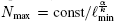 . A possible situation could be that k = α, then a linear decrease in the chip technology will yield an increase in the maximum size. A better situation is when k ≪ α since then the improvement will be over previous pay off. However, the worst situation occurs when k ≫ α. In the limit case of k → ∞, the maximum size would be insensitive to any technological improvement.
Therefore, a practical criterion for the class P is to compare the integer k with the technological scaling exponent α, i.e. k vs. α, rather than the more theoretical criterion of comparing k vs. ∞.
Another important practical case we may face is the existence of technological barriers. For example, today computer technology has reached the nanometre scale. Suppose we have a certain set of data like (31) obtained with a class P algorithm, but we need to increase the maximum size by a factor ƒ > 1 such that then we need to go down well beyond the size of angstroms. Then, for those smaller sizes, the computer leaves the classical behaviour and enter the realm of quantum mechanics, so that we may well need a quantum computer to expand the range of data and be able to find our law.
B. On the Halting Problem in Chess
The halting problem has many implications as we have shown. It is a concept of practical use in games, particularly in advanced games like chess. There, it is important to make sure that the rules of the game (axioms) will ensure that the match will terminate. Until 1929, players were not aware that the set of rules already known made it possible to produce never-ending chess matches. In that year, Max Euwe, a mathematician later to become the fifth world chess champion of modern history 1935-37, settled the question by rediscovering the Thue-Marston (Thue, 1906Thue, A. (1906). "Fiber unendliche Zeichenreihen". Norske vid. Selsk. Skr. Mat. Nat. Kl., 7, pp. 1-22, Reprinted in Selected Mathematical Papers of Axel Thue (Ed. T. Nagell). Oslo: Universitetsforlaget, pp. 139-158, 1977. M. Morse, “Recurrent Geodesics on a Surface of Negative Curvature.” Trans. Amer. Math. Soc. 22, 84-100, (1921).) sequence and its cube-free property.
In binary language, the Thue-Marston sequence is defined by the following generating moves:
For instance, the first elements of the sequence are
An element of a sequence is cube-free if it contains no subsequence of the form ppp, where p is a finite non-empty element.
A chess match is divided in three parts: opening, middle-game and end-game. The end-game is characterized by the presence of very few pieces on the board compared to the opening. Thus, a theory of the end-game in chess is highly developed as its complexity is reduced. It had been known that repetition of movements, a loop, may happen in certain situations. Rules were established to declare a draw when repetition of moves become endless. Euwe (Euwe, 1929Euwe, M. (1929). "Mengentheoretische Betrachtungen über das Schachspiel". Proc. Konin. Akad. Wetenschappen (Amsterdam), 32 (5), pp. 633-642.) used the cubic-free property of the Thue-Marston sequence to show how to circumvent those rules. Thus, new rules had to be added to the game. This is another instance of how axioms, i.e. rules, may be changed a posteriori depending on the type of theory we want to have.
When Bobby Fischer was an active chess player, he would say “Gods put the middle game after the opening”, meaning that the complexity of the middle game was so high that it was unknown territory, where written manuals for openings were useless, and he would feel at his best. After retirement, in the 1980’s Fischer sent a warning call saying that chess was becoming too technical, mechanical and with little room for creativity. He proposed to change the rules of the opening somehow, interestingly enough, introducing some randomness in chess. In particular, by randomizing the starting position of the main pieces in the first row of each player side. And this happened way before a computer, Deep Blue, defeated the World Chess Champion G. Kasparov in 1997. Many people thought this to be unbelievable before year 2000. This does not mean that computers are more intelligent than us, or intelligent at all. It means that their brute force of calculation is stronger than ours at playing chess.
C. Divertimento: On the Complexity of Music
Mozart composed many divertimentos, a musical form very common in the Classical era prior to the success of the sonata form by Haydn. We may produce a divertimento playing with Turing’s ideas in music.
Music is more than a language, but insofar as it is a language, we can apply Turing’s results to it and prove some amusing results which may surprise music theorists, particularly given that they can be proved mathematically.
i/ There is an endless number of different musical compositions.
ii/ There are musical compositions that cannot be composed.
Statement i/ implies that musical creativity is infinite, for sure, while ii/ means that, nevertheless, it also has some limits.
To proof i/ we use a code such that the music symbols and rules of composition are encoded with a given alphabet  . This can be binary for instance. Then, we use the same code alphabet to label all known compositions. This can be done by lexicographic order, forming a table like (7). Now, applying the diagonal method we obtain another composition which is certain to be new. Though it is unlikely that these mathematical type of compositions would have pleased Mozart and Haydn, it may produce a different reaction in B. Bartók, A. Schongberg, J. Cage, G. Ligeti, K. Stockhausen, I. Xenakis, P. Boulez, C. Halffter... Nevertheless, what is remarkable, and unimaginable before Turing, is that a computer could be of help as a composition machine as they are used nowadays.
To prove ii/ we need to realize that each music composition is like a TM. Thus, it may or may not halt. For instance, we can produce simple scores that repeat themselves forever. Accepting this proviso about endless compositions is essential. Suppose now that we want to write a music composition that with our language would be equivalent to a program that finds when any other musical composition will ever halt. Then, that score is impossible to be written.
Cellular automata are used to produce musical scores (Wolfram, 2002Wolfram, S.Wolfram Tones (2002). Retrieved from http://tones.wolfram.com/.; Millen, 1990Millen, D. (1990). "Cellular Automata Music". In International Computer Music Conference. Glasgow, Retrieved from http://comp.uark.edu/dmillen/cam.html.; Bozkurt, 2011Bozkurt, B. (2011). Otomata - Online Generative Musical Sequencer, Retrieved from http://www.earslap.com/projectslab/otomata.), and some them are equivalent to a universal Turing machine, like the Rule 110 cellular automaton (Cook, 2004Cook, M. (2004). "Universality in Elementary Cellular Automata". Complex Systems, 15, pp. 1-40.).
In the early 20th century, Arnold Schongberg evaluated the situation of classical music and judged that the tonal system based on major and minor scales, Greek modes etc. was absolutely worn out. Subjective as this may be, he went on to search for new composition systems by relaxing the rigidities of the old system. For instance, allowing all tones in a dodecaphonic scale to play the same role, without dominant or tonic tones. This produce non-tonal systems like the twelve-tone method and many others to follow, even by introducing random methods and other tools from Mathematics, like set theory. Again, that situation arose because creativity was judged to be exhausted, and a change or extension of axioms was proposed instead, leading to controversy. Nevertheless, controversy is unavoidable here since music is more than a language and personal taste plays a major role.
VIII. CONCLUSIONS Top
Turing revolutionized the fundamental roots of what we understand by scientific knowledge, and he will continue to do so as many new applications of his works arise. At the same time, his scientific work still lacks the recognition that it deserves in his own field of Mathematics. As he also founded modern computer science, recognition came first mainly from Engineering and Physics.
The part of Turing’s 1936 paper (Turing, 1936Turing, A. M. (1936). "On computable numbers, with an application to the Entscheidungsproblem". Proc. London Math. Soc., {[2]} 42 (1936-37), 230-265; Correction, ibid., 43 (1937), 544-546. Online open access http://www.abelard.org/turpap2/tp2-ie.asp.) devoted to computable numbers has given rise to the development of computer technology as a whole. This is having a gigantic impact on our culture. The other part of Turing’s paper devoted to the solution of Hilbert’s tenth problem, as a consequence of the previous one, has helped us to deepen our knowledge about scientific knowledge itself. This is best exemplified by the work of Chaitin, who has formalized what is knowable and unknowable based on Turing’s work, and extending Godel’s results in a more systematic and accessible way. His conclusion is somewhat shocking as it implies that logical randomness is common even in Mathematics.
There is a parallelism between intrinsic randomness in Mathematics and in Physics, and we can learn from it. In Physics it appeared in the 1920’s in Quantum Mechanics, and also produced a shocking revolution that removed the holy grail of classical Physics, determinism, from the central status it had been enjoying. Nowadays, Quantum Mechanics is a successful theory and has been accepted both logically and empirically, due to unprecedentedly accurate experimental results. In Mathematics, logical randomness appeared in 1930’s and is also becoming accepted.
After the work of Gödel, Turing and Chaitin it is certain that a TOE of Mathematics is impossible. But, what about Physics? Inasmuch as Physics inherits the language of Mathematics to express its laws and work out its consequences, we may immediately deduce that the same applies to Physics and there is no TOE for it. However, Physics is more than a language and the ultimate word relies on experience, on the natural law. Our physical knowledge is like a window on an energy scale, ranging from some point in the infrared to some point in the ultraviolet, i.e., large distance scales to small distance scales. From this finite window scale we may bet on two possibilities: i/ that no TOE of Physics exists, since as we enlarge the energy window we will get new laws of Physics that were not anticipated; ii/ that a TOE of Physics do exists and from our current window of knowledge, or probably a better one, we can deduce the whole range of physical laws in the entire energy scale, i.e., Physics would be finite and closed as a source of knowledge. Following Turing’s work, I believe that option i/ is the correct one, and experience will tell us. The non-existence of a TOE in Physics is good news for creativity in contrast to reductionism.
Is it true that true randomness is only quantum? The Ω number is a real number whose binary expansion yields bits of information that are true for no reason, they have no structure or pattern, it is incompressible and its bits totally random as Chaitin has shown.
The following question may help to face this outcome situation not so dramatically. How can it be that Natural Sciences like Physics, Mathematics, etc have become so successful if we live in a world plagued by intrinsic randomness? A clue to this question is to take the example of what type of real numbers are employed in successful theories. We will see that we always have real numbers like √2, π, e, etc. Although they are irrational with an infinite number of decimals, we have very short algorithms that generate that series of decimals very efficiently. I.e., they are actually maximally compressible numbers.
This fact can be extrapolated to the whole structure of successful theories of Nature: they are very simple, they can be compressed, reduced to a simple set of axioms or laws of Nature. The rest of the universe that remains unknown is due in part because it is not compressible and we live in a small region of the whole space of theories or knowledge. We may divide our ‘sphere of knowledge’ into three parts: i/ current science (known); ii/ future science (to be known); and iii/ unknowable or irreducible.
Physicists are willing to find and adopt new physical principles, laws that expand their knowledge of the universe. Mathematicians, standard and formal ones, tend to stick rigidly to axioms and not to modify them. They should adopt a more experimental attitude. With Turing, the fields of Mathematics and Physics become more unified.
ACKNOWLEDGMENTS
Top
M.A.M.-D. thanks the Spanish MICINN grant F15200910061, CAM research consortium QUITEMAD 52009-ESP1594, European Commission PICC: FP7 2007-2013, Grant No. 249958, UCM-BS grant GICC-910758.
REFERENCESTop
|
| ○ | Aaronson, S.; Kuperberg, G. and Granade, C. (2005). The Complexity Zoo, retrieved from https://complexityzoo.uwaterloo.ca/ComplexityZoo. |
| ○ | Association for Computing Machinery (2001). Retrieved from http://awards.acm.org/. |
| ○ | Bernstein, E. and Vazirani, U. (1997). "Quantum complexity theory". SIAM J. Comput., 26, pp. 1411-1473. |
| ○ | Berthiaume, A.; van Dam, W. and Laplante, S. (2000). Quantum Kolmogorov Complexity, arXiv: retrieved from quant-ph/005018. |
| ○ | Borel, E. (1909). "Les probabilités dénombrables et leurs applications arithmétiques". Rendiconti del Circolo Matematico di Palermo, 27, pp. 247-271. |
| ○ | Borel, E. (1952). Les nombres inaccessibles. Paris: Ed. Gauthier-Villars, 10+141 pp. |
| ○ | Bozkurt, B. (2011). Otomata - Online Generative Musical Sequencer, Retrieved from http://www.earslap.com/projectslab/otomata. |
| ○ | Chaitin, G. J. (1966). "On the length of programs for computing finite binary sequences". Journal of the ACM, 13, pp. 547-569. |
| ○ | Chaitin, G. J. (1975). "A theory of program size formally identical to information theory". J. ACM, 22, pp. 329-340. |
| ○ | Chaitin, G. J. (1987). Algorithmic Information Theory. Cambridge University Press. |
| ○ | Chaitin, G. J. (2001). Exploring randomness. London: Springer-Verlag. |
| ○ | Chaitin, G. J. (2003). The Limits of Mathematics. London: Springer-Verlag. |
| ○ | Chaitin, G. J. (2009). "Leibniz, Complexity and Incompleteness". APA Newsletter on Philosophy and Computers, 9 (1), pp. 7-10. |
| ○ | Chaitin, G. J. (2011). "To a mathematical theory of evolution and biological creativity"; preprint. Paper presented Monday 10 January 2011 at a workshop on “Randomness, Structure and Causality: Measures of Complexity from Theory to Applications” organized by Jim Crutcheld and Jon Machta at the Santa Fe Institute in New Mexico. |
| ○ | Chaitin, G. J. (2012). Proving Darwin. New York: Pantheon. |
| ○ | Chaitin, G. J. (2012b). "Life as evolving software". In Zenil, H. (ed.), A Computable Universe. Singapore: World Scientific. |
| ○ | Calude, C. S. (2002). Information and Randomness. An Algorithmic Perspective. Second Edition. Berlin, Heidelberg, New York: Springer-Verlag. |
| ○ | Calude, C. S.; Dinneen, M. J. and Shu, C.-K. (2002). "Computing a glimpse of randomness". Exper. Math., 11, pp. 361-370. |
| ○ | Calude, C. S. and Pavlov, B. (2002). "Coins, Quantum Measurements, and Turing’s Barrier". Quantum Information Processing, 1 (1-2). |
| ○ | Cover, T. M. and Thomas, J. A. (2006). Elements of Information Theory. Second Edition. New Jersey: John Wiley & Sons, Inc. |
| ○ | Cantor, G. (1891). See (Suppes, 1960). |
| ○ | Cohen, P. J. (1963). "The Independence of the Continuum Hypothesis". Proceedings of the National Academy of Sciences of the United States of America, 50 (6), pp. 1143-1148. |
| ○ | Collatz, L. (1937). Unpublished. |
| ○ | Cook, M. (2004). "Universality in Elementary Cellular Automata". Complex Systems, 15, pp. 1-40. |
| ○ | Copeland, J. and Proudfoot, D. (1999). "Alan Turing’s forgotten ideas in computer science". Scientific American, April issue. |
| ○ | Copeland, J. (ed.) (2004). The Essential Turing: Seminal Writings in Computing, Logic, Philosophy, Artificial Intelligence, and Artificial Life plus The Secrets of Enigma. Oxford, UK: Clarendon Press (Oxford University Press). |
| ○ | Dauben, J. W. (1979). Georg Cantor: his mathematics and philosophy of the infinite. Boston: Harvard University Press. |
| ○ | Davis, M. (1958). Computability and Unsolvability. New York: McGraw-Hill. |
| ○ | De las Cuevas, G.; Dür, W.; Van den Nest, M. and Martin-Delgado, M. A. (2011). "Quantum algorithms for classical lattice models". New J. of Physics, 13:093021, arXiv:1104.2517. |
| ○ | Euwe, M. (1929). "Mengentheoretische Betrachtungen über das Schachspiel". Proc. Konin. Akad. Wetenschappen (Amsterdam), 32 (5), pp. 633-642. |
| ○ | Feynman, R. P. (1982). "Simulating physics with computers". Int. J. Theor. Phys., 21, pp. 467-488. |
| ○ | Gács, P. (2000). "Quantum Algorithmic Entropy". J. Phys. A: Math. Gen., 34, (2001). arXiv: retrieved from http://arxiv.org/abs/quant-ph/0011046v2. |
| ○ | Galindo, A. and Martin-Delgado, M. A. (2002). "Information and Computation: Classical and Quantum Aspects". Rev.Mod.Phys., 74, pp. 347-423. arXiv: quant-ph/0112105. |
| ○ | Gödel, K. F. (1931). "Fiber formal unentscheidbare Sátze der Principia Mathematica and verwandter Systeme, I". Monatshefte für Mathematik and Physik, 38, pp. 173-98. |
| ○ | Gödel, K. F. (1940). The Consistency of the Axiom of Choice and of the Generalized Continuum Hypothesis with the Axioms of Set Theory. Princeton University Press. |
| ○ | Hilbert, D. (1927). "The foundations of mathematics". translated by Stephan Bauer-Menglerberg and Dagfinn Follesdal (pp. 464-479). In van Heijenoort, J. (1967, 3rd printing 1976) (ed.), From Frege to Godel: A Source Book in Mathematical Logic. Cambridge, MA: Harvard University Press, pp. 1879-1931. |
| ○ | Kieu, T. D. (2003). Quantum Algorithm for Hilbert’s Tenth Problem, retrieved from arXiv:quant-ph/0310052v2. |
| ○ | Knuth, D. E. (2000). Selected Papers on Analysis of Algorithms. Stanford, California: Center for the Study of Language and Information - CSLI Lecture Notes, no. 102. |
| ○ | Kolmogorov, A. N. (1965). "Three Approaches to the Quantitative Definition of Information". Problems Inform. Transmission, 1 (1), pp. 1-7. |
| ○ | Kurtz, S. A. and Simon, J. (2007). "The Undecidability of the Generalized Collatz Problem". In Cai, J.-Y.; Cooper, S.B. and Zhu, H. (eds.), Proceedings of the 4th International Conference on Theory and Applications of Models of Computation, TAMC 2007, held in Shanghai, China in May 2007, pp. 542-553. |
| ○ | Leibniz, G. W. (1686). Discours de métaphysique. |
| ○ | Li, M. and Vitanyi, P. (1990). "Kolmogorov complexity and its applications". In van Leeuven, J. (ed.), Handbook of Theoretical Computer Science, Vol. A, pp. 187-254. |
| ○ | Martin-Delgado, M. A. (2011). "On Quantum Effects in a Theory of Biological Evolution". Scientific Reports, 2, 302, (2012). Retrieved from arxive arXiv:1109.0383. |
| ○ | Martin-Löf, P. (1966). "The Definition of Random Sequences". Information and Control, 9 (6), pp. 602-619. |
| ○ | Millen, D. (1990). "Cellular Automata Music". In International Computer Music Conference. Glasgow, Retrieved from http://comp.uark.edu/dmillen/cam.html. |
| ○ | Minsky, M. L. (1962). "Size and Structure of Universal Turing Machines Using Tag Systems". Proc. Sympos. Pure Math., 5, pp. 229-238. |
| ○ | Moore, G. E. (1965). "Cramming more components onto integrated circuits". Electronics, 38 (8), April 19. |
| ○ | Mora, C. and Briegel, H. J. (2004). "Algorithmic complexity of quantum states", retrieved from arXiv:quantph/0412172. |
| ○ | Mora, C. and Briegel, H. J. (2005). "Algorithmic complexity and entanglement of quantum states". Phys. Rev. Lett., 95 (20). |
| ○ | Mora, C.; Briegel, H. J. and Kraus, B. (2006). "Quantum Kolmogorov complexity and its applications", retrieved from arXiv: quant-ph/0610109. |
| ○ | Newton, I. (1687). Philosophiae Naturalis Principia Mathematica. London Online version: http://www.ntnu.no/ub/spesialsamlingene/ebok/02a019654.html. |
| ○ | Oliveira e Silva, T. (2012). Retrieved from http://www.ieeta.pt/ tos/3x+1.html. |
| ○ | Radó, T. (1962). "On non-computable functions". Bell System Technical Journal, 41 (3), pp. 877-884. |
| ○ | Rogozhin, Y. (1996). "Small Universal Turing Machines". Theoret. Comput. Sci., 168, pp. 215-240. |
| ○ | Shannon, C. E. (1956). "A Universal Turing Machine with Two Internal States". In Automata Studies. Princeton, NJ: Princeton University Press, pp. 157-165. |
| ○ | Solomonoff, R. (1964). "A Formal Theory of Inductive In¬ference Part I". Information and Control, 7 (1), pp. 1-22. |
| ○ | Suppes, P. (1972, 1960). Axiomatic Set Theory. New York: Dover. |
| ○ | Svozil, K. (1995). "Quantum algorithmic information theory", eprint arXiv:quant-ph/9510005. |
| ○ | Svozil, K. (1995b). "Halting probability amplitude of quantum computers". Journal of Universal Computer Science, 1 (3). |
| ○ | Turing, A. M. (1936). "On computable numbers, with an application to the Entscheidungsproblem". Proc. London Math. Soc., {[2]} 42 (1936-37), 230-265; Correction, ibid., 43 (1937), 544-546. Online open access http://www.abelard.org/turpap2/tp2-ie.asp. |
| ○ | Turing, A. M. (1946). "Proposed Electronic Calculator" (ACE), National Physical Laboratory internal document (1946). The original copy is in the (British) National Archives, in the file DSIR 10/385. first published as the NPL report, Com. Sci. 57 (1972), with a foreword by Donald W. Davies. |
| ○ | Thue, A. (1906). "Fiber unendliche Zeichenreihen". Norske vid. Selsk. Skr. Mat. Nat. Kl., 7, pp. 1-22, Reprinted in Selected Mathematical Papers of Axel Thue (Ed. T. Nagell). Oslo: Universitetsforlaget, pp. 139-158, 1977. M. Morse, “Recurrent Geodesics on a Surface of Negative Curvature.” Trans. Amer. Math. Soc. 22, 84-100, (1921). |
| ○ | Van den Nest, M.; Dür, W.; Raussendorf, R. and Briegel, H. J. (2009). "Quantum algorithms for spin models and simulable gate sets for quantum computation". Phys. Rev. A, 80, 052334. |
| ○ | Vitanyi, P. (2000). "Three Approaches to the Quantitative Definition of Information in an Individual Pure Quantum State", arXiv: retrieved from quant-ph/9907035. |
| ○ | Weyl, H. (1927). Philosophy of Mathematics and Natural Science, translated by Olaf Helmer with a new introduction by Franck Wilczek. Princeton University Press, New Jersey (1949). Parts of this book were originally published by R. Oldenbourg in German in 1927 in Handbuch der Philosophie under the title “Philosophie der Mathematik and Naturwis-senschaft". |
| ○ | Wolfram, S. (2002). Wolfram Tones. Retrieved from http://tones.wolfram.com/. |
| ○ | Yao, A. (1993). Proceedings of the 34th IEEE Symposium on the Foundations of Computer Science, (IEEE Computer Society, Los Alamitos, CA), p. 352. |
|